Agentic forecasting with skforecast-ai¶

What is skforecast-ai?¶

skforecast-ai is an AI forecasting assistant that pairs a deterministic engine, powered by skforecast, with an LLM reasoning layer. Simply provide a time series, and the assistant automatically profiles the data, selects a model using established best practices, and evaluates its performance. It returns both the final forecast and the runnable skforecast script that produced it.

It is organized around a single core object, the ForecastingAssistant, which consists of two complementary components:

• Deterministic Engine (Rule-based and Reproducible): Profiles the data, selects a forecaster and estimator, derives lags and preprocessing steps, runs backtesting, and produces the final forecast. Crucially, it outputs the exact standalone skforecast script that generated the results. Given the same inputs and configuration, this workflow is guaranteed to be reproducible.

• Reasoning Layer (LLM-powered): Accessed primarily via the ask() method, this layer interprets and explains the objects and results you pass to it: data profiles, modeling plans, validation choices, backtesting outputs, and forecasts. The LLM acts strictly as an interpreter; it does not rerun the workflow or silently change modeling recommendations behind the scenes. Agentic features, such as the LLM-guided refine_plan() or create_cv(), are separate, explicit steps where the LLM suggests adjustments that are then implemented transparently in deterministic code.

Two ways to use skforecast-ai¶

skforecast-ai supports two distinct workflows using the same underlying forecasting engine:

• The Fast Path: Use this when you want a forecast or backtest result in a single call. The assistant profiles the data, builds the modeling plan, executes the workflow, and returns the results alongside the reproducible skforecast code.

• The Step-by-Step Path: Use this when you want granular control to inspect or adjust intermediate decisions. You can manually create a profile, build a plan, optionally refine it with the LLM, define a validation strategy, evaluate the model, and then generate the forecast.

A useful mental model is that forecasting and validation are separate branches. Once you have a profile and a plan, you can use forecast() to produce future predictions directly, or backtest() to evaluate the model's performance on historical data.

The ask() method is available in both workflows. It can explain a profile, plan, validation setup, backtest result, or answer general forecasting questions, but it will never execute the workflow or modify your parameters without explicit instruction.

Fast path: one call

Profiling, planning and execution happen internally.

data

↓

Forecast

forecast()
or forecast_code()

↓

predictions + code

Backtesting (validation)

create_cv()
Deterministic, Agentic mode
or pass a skforecast TimeSeriesFold object

↓

backtest()
or backtest_code()

↓

metrics + predictions + code

Step-by-step path: full control

Build a profile and a plan from your data, then branch into forecasting and backtesting.

data

↓

profile()

↓

plan()
refine_plan(), optional (Deterministic or Agentic mode)

↓

Forecast

forecast()
or forecast_code()

↓

predictions + code

Backtesting (validation)

create_cv()
Deterministic, Agentic mode
or pass a skforecast TimeSeriesFold object

↓

backtest()
or backtest_code()

↓

metrics + predictions + code

LLM reasoning: available at any moment, in any workflow

Call ask() before, during or after either path. It can take a profile, a plan, a forecast_result, a backtest_result, or nothing at all (pure Q&A).

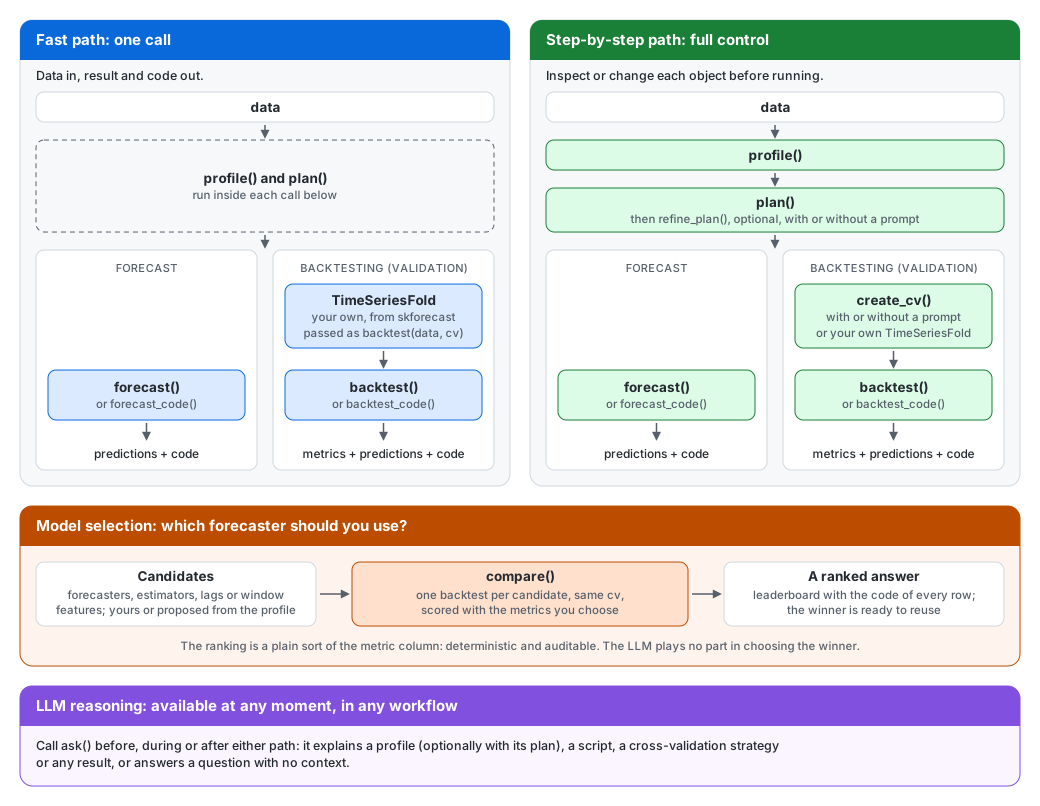
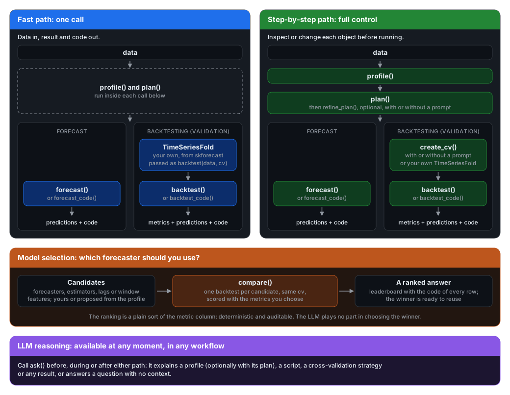
The following example walks through the fast path: the quickest way to go from raw data to a validated forecast with minimal setup. It is ideal when you want rapid results and trust the assistant to make sensible, baseline modeling decisions on your behalf. If you prefer to understand and control what happens under the hood step by step, visit the step-by-step path tutorial for a more detailed walkthrough.

Assistant initialization¶

The first step is to instantiate a ForecastingAssistant, which will be responsible for executing the entire workflow (profiling, planning, backtesting, and forecasting), as well as explaining the outputs and suggesting improvements.

To activate the optional LLM support, users must pass a string in the format 'provider:model_name' (for example, 'openai:gpt-5.5', 'google:gemini-3-flash-preview', 'anthropic:claude-sonnet-5', or 'ollama:qwen3:8b'). For hosted providers, the corresponding API key must be available as an environment variable or passed explicitly when creating the assistant. In this tutorial, we set send_data_to_llm=False. This ensures strict data privacy: the LLM receives only metadata and summary statistics, never the raw time series values.

In [11]:

# Data processing
# ==============================================================================
import os
import numpy as np
import pandas as pd
from skforecast.datasets import fetch_dataset

# Plots
# ==============================================================================
from skforecast.plot import set_dark_theme
import matplotlib.pyplot as plt
import plotly.graph_objects as go
import plotly.io as pio
import plotly.offline as poff
pio.templates.default = "seaborn"
poff.init_notebook_mode(connected=True)
plt.style.use('seaborn-v0_8-darkgrid')

# skforecast and skforecast-ai
# ==============================================================================
import skforecast
import skforecast_ai
from skforecast_ai import ForecastingAssistant
from skforecast.model_selection import TimeSeriesFold

color = '\033[1m\033[38;5;208m' 
print(f"{color}Version skforecast_ai: {skforecast_ai.__version__}")
print(f"{color}Version skforecast: {skforecast.__version__}")

# Data processing # ============================================================================== import os import numpy as np import pandas as pd from skforecast.datasets import fetch_dataset # Plots # ============================================================================== from skforecast.plot import set_dark_theme import matplotlib.pyplot as plt import plotly.graph_objects as go import plotly.io as pio import plotly.offline as poff pio.templates.default = "seaborn" poff.init_notebook_mode(connected=True) plt.style.use('seaborn-v0_8-darkgrid') # skforecast and skforecast-ai # ============================================================================== import skforecast import skforecast_ai from skforecast_ai import ForecastingAssistant from skforecast.model_selection import TimeSeriesFold color = '\033[1m\033[38;5;208m' print(f"{color}Version skforecast_ai: {skforecast_ai.__version__}") print(f"{color}Version skforecast: {skforecast.__version__}")

Version skforecast_ai: 0.1.0
Version skforecast: 0.23.0

✏️ Note

If you do not have access to an LLM assistant, you can still follow the full tutorial using only the deterministic methods. Profiling, planning, backtesting, and forecasting all run without an LLM. Only the ask() explanations and the LLM-guided variants of refine_plan() and create_cv() require a configured LLM; their deterministic counterparts (for example, refine_plan() with explicit overrides and prompt=None) work without one.

In [ ]:

# LLM-enabled assistant
# ==============================================================================
LLM_MODEL = "google:gemini-3-flash-preview"
api_key = os.getenv("GOOGLE_API_KEY")

assistant = ForecastingAssistant(
    llm=LLM_MODEL, api_key=api_key, send_data_to_llm=False
)

# Using aws bedrock
# ==============================================================================
# assistant = ForecastingAssistant(
#     llm='bedrock:eu.anthropic.claude-sonnet-4-6',
#     base_url="eu-west-1"
# )

# Assistant without reasoning layer
# ==============================================================================
# assistant = ForecastingAssistant()

# LLM-enabled assistant # ============================================================================== LLM_MODEL = "google:gemini-3-flash-preview" api_key = os.getenv("GOOGLE_API_KEY") assistant = ForecastingAssistant( llm=LLM_MODEL, api_key=api_key, send_data_to_llm=False ) # Using aws bedrock # ============================================================================== # assistant = ForecastingAssistant( # llm='bedrock:eu.anthropic.claude-sonnet-4-6', # base_url="eu-west-1" # ) # Assistant without reasoning layer # ============================================================================== # assistant = ForecastingAssistant()

⚠️ Your data stays private

By default, enabling an LLM does not send your time-series data to the model provider. The assistant passes only summary statistics, detected frequency, seasonality flags and the forecaster configuration, never the raw observations. To explicitly allow it, pass send_data_to_llm=True.

Data¶

The data in this document represent the hourly usage of the bike share system in the city of Washington, D.C. during the years 2011 and 2012. In addition to the number of users per hour, information about weather conditions and holidays is available.

In [13]:

# Downloading data
# ==============================================================================
data = fetch_dataset('bike_sharing', raw=True)
data = data[['date_time', 'users', 'holiday', 'weather', 'temp']]
data.head()

# Downloading data # ============================================================================== data = fetch_dataset('bike_sharing', raw=True) data = data[['date_time', 'users', 'holiday', 'weather', 'temp']] data.head()

╭───────────────────────────────── bike_sharing ──────────────────────────────────╮
│ Description:                                                                    │
│ Hourly usage of the bike share system in the city of Washington D.C. during the │
│ years 2011 and 2012. In addition to the number of users per hour, information   │
│ about weather conditions and holidays is available.                             │
│                                                                                 │
│ Source:                                                                         │
│ Fanaee-T,Hadi. (2013). Bike Sharing Dataset. UCI Machine Learning Repository.   │
│ https://doi.org/10.24432/C5W894.                                                │
│                                                                                 │
│ URL:                                                                            │
│ https://raw.githubusercontent.com/skforecast/skforecast-                        │
│ datasets/main/data/bike_sharing_dataset_clean.csv                               │
│                                                                                 │
│ Shape: 17544 rows x 12 columns                                                  │
╰─────────────────────────────────────────────────────────────────────────────────╯

Out[13]:

	date_time	users	holiday	weather	temp
0	2011-01-01 00:00:00	16.0	0.0	clear	9.84
1	2011-01-01 01:00:00	40.0	0.0	clear	9.02
2	2011-01-01 02:00:00	32.0	0.0	clear	9.02
3	2011-01-01 03:00:00	13.0	0.0	clear	9.84
4	2011-01-01 04:00:00	1.0	0.0	clear	9.84

✏️ Note

skforecast-ai is ready to preprocess the data, but it is recommended that users apply their own preprocessing steps before using the assistant. This ensures the data is in the desired format and any necessary transformations have been applied before proceeding with the forecasting workflow.

In [14]:

# Interactive plot of time series
# ==============================================================================
fig = go.Figure()
fig.add_trace(
    go.Scatter(x=data['date_time'], y=data['users'], mode='lines', name='Train')
)
fig.update_layout(
    title  = 'Number of users',
    xaxis_title="Time",
    yaxis_title="Users",
    legend_title="Partition:",
    width=800,
    height=400,
    margin=dict(l=20, r=20, t=35, b=20),
    legend=dict(orientation="h", yanchor="top", y=1, xanchor="left", x=0.001)
)
fig.show()

# Interactive plot of time series # ============================================================================== fig = go.Figure() fig.add_trace( go.Scatter(x=data['date_time'], y=data['users'], mode='lines', name='Train') ) fig.update_layout( title = 'Number of users', xaxis_title="Time", yaxis_title="Users", legend_title="Partition:", width=800, height=400, margin=dict(l=20, r=20, t=35, b=20), legend=dict(orientation="h", yanchor="top", y=1, xanchor="left", x=0.001) ) fig.show()

For a deeper walkthrough of the exploratory analysis behind this dataset, see the skforecast example: Forecasting time series with skforecast, XGBoost, LightGBM and CatBoost.

Forecasting with the assistant¶

The forecast() method is the fastest way to generate predictions. In a single call, it executes the full pipeline (profile → plan → execute) and returns a ForecastResult holding the predictions, the evaluation metrics (when available), and the exact standalone skforecast script that produced them.

The behavior is controlled by a single switch, test_size, which selects one of two modes:

• Prediction mode (test_size = None, the default): The model is trained on the entire dataset and forecasts the next steps time points into the future. Because there is no ground truth to compare against, no metrics are returned. If the historical data contains exogenous variables, their future values must be explicitly supplied via the exog argument.

• Evaluation mode (test_size is set). The dataset is split into train and test sets, the model is trained on the training portion, and predictions for the test window are compared against the held-out actuals to compute metrics. In this mode, the test-set exogenous values are taken from the split, so exog must not be passed.

The main arguments are:

Argument	Type	Description
data	Series, DataFrame, str, Path	Input dataset or path to a CSV file. When a Series is passed, the target is taken from its name.
steps	int	Forecast horizon (number of steps ahead to predict).
target	str, list of str	Column to forecast. Optional when data is a Series. Pass a list of column names for wide-format multi-series.
date_column	str	Column holding the timestamps. When None, the index of data must already be a DatetimeIndex.
exog	DataFrame	Future exogenous values covering the horizon (at least steps rows). Used only in prediction mode, and required there when the data has exogenous variables.
interval	list of float	Prediction interval as [lower, upper] quantiles (e.g. [0.1, 0.9] for an 80% interval). None disables intervals.
test_size	int, float, str, Timestamp	Size or start of the test set, selecting the mode above. int: last test_size observations; float in (0, 1): last fraction of observations; str/Timestamp: first timestamp of the test set. None runs prediction mode.

💡 Tip

You can also use custom configurations for the forecaster, estimator, estimator_kwargs, lags, and window_features by passing them as arguments to forecast(). This allows you to override the assistant's automatic choices and use your own preferred settings. For example, this code specifies a custom forecaster while still letting the assistant handle the rest of the workflow:

results = assistant.forecast(
              data        = data,
              target      = 'users',
              date_column = "date_time",
              steps       = 36,
              forecaster  = 'ForecasterFoundation'
          )

The following code demonstrates how to execute the assistant in evaluation mode. By explicitly defining the test_size parameter (in this case, test_size=36), the pipeline automatically reserves the final 36 observations as a test set.

During execution, the assistant profiles the dataset, incorporates the provided exogenous features (holiday, weather, and temp), and trains an appropriate model on the training split. Because the method is triggered in evaluation mode, the resulting ForecastResult object provides the out-of-sample predictions, an 80% prediction interval, and the performance metrics evaluated against the held-out ground truth.

In [15]:

# Execute the forecasting assistant in evaluation mode
# ==============================================================================
results = assistant.forecast(
              data        = data,
              target      = 'users',
              date_column = "date_time",
              steps       = 36,
              interval    = [0.1, 0.9],  # 80% prediction interval
              test_size   = 36           # Last 36 hours as test set (evaluation mode)
          )

# Execute the forecasting assistant in evaluation mode # ============================================================================== results = assistant.forecast( data = data, target = 'users', date_column = "date_time", steps = 36, interval = [0.1, 0.9], # 80% prediction interval test_size = 36 # Last 36 hours as test set (evaluation mode) )

In [16]:

# Inspect the performance metrics and the resulting predictions
# ==============================================================================
display(results.metrics)
display(results.predictions.head())

# Inspect the performance metrics and the resulting predictions # ============================================================================== display(results.metrics) display(results.predictions.head())

	series	MAE	MSE	MASE	MAPE
0	users	30.192265	2527.408894	0.468903	0.410562

	pred	lower_bound	upper_bound
2012-12-30 12:00:00	149.399731	120.100076	180.936632
2012-12-30 13:00:00	136.393947	102.712610	186.309126
2012-12-30 14:00:00	138.424149	100.203602	186.527043
2012-12-30 15:00:00	147.257449	109.043734	190.882050
2012-12-30 16:00:00	143.084084	100.749418	181.536869

The show_code() method allows users to retrieve the exact code used to generate the forecast.

In [17]:

# skforecast code that generated the results
# ==============================================================================
results.show_code()

# skforecast code that generated the results # ============================================================================== results.show_code()

Generated codeCopy

import pandas as pd                                                                       
from sklearn.metrics import mean_absolute_error, mean_squared_error,                      
mean_absolute_percentage_error                                                            
from skforecast.metrics import mean_absolute_scaled_error                                 
from lightgbm import LGBMRegressor                                                        
from skforecast.preprocessing import RollingFeatures, CalendarFeatures                    
from skforecast.recursive import ForecasterRecursive                                      
                                                                                          
# Load data                                                                               
data = pd.read_csv('data.csv')                                                            
                                                                                          
data['date_time'] = pd.to_datetime(data['date_time'])                                     
data = data.set_index('date_time')                                                        
data = data.asfreq('h')                                                                   
data = data.sort_index()                                                                  
                                                                                          
# Train/test split                                                                        
end_train = '2012-12-30 11:00:00'  # last training date, adjust to change the split point 
data_train = data.loc[:end_train]                                                         
data_test  = data.loc[data.index > end_train]                                             
exog_features = ['holiday', 'weather', 'temp']                                            
                                                                                          
print(                                                                                    
    f"Train dates : {data_train.index.min()} --- {data_train.index.max()}                 
(n={len(data_train)})"                                                                    
)                                                                                         
print(                                                                                    
    f"Test dates  : {data_test.index.min()} --- {data_test.index.max()}                   
(n={len(data_test)})"                                                                     
)                                                                                         
                                                                                          
window_features = RollingFeatures(                                                        
    stats        = ['mean', 'std', 'mean', 'mean'],                                       
    window_sizes = [3, 3, 24, 168],                                                       
)                                                                                         
                                                                                          
calendar_features = CalendarFeatures(                                                     
    features = ['hour', 'day_of_week', 'weekend', 'month'],                               
    encoding = None,                                                                      
)                                                                                         
                                                                                          
# Create forecaster                                                                       
forecaster = ForecasterRecursive(                                                         
    estimator            = LGBMRegressor(random_state=123, verbose=-1),                   
    lags                 = [1, 2, 3, 5, 8, 10, 15, 17, 19, 20, 21, 22, 23, 24, 25, 26, 32,
33, 119, 121, 135, 136, 142, 143, 145, 160, 166, 167, 169, 313, 335, 337],                
    window_features      = window_features,                                               
    calendar_features    = calendar_features,                                             
    categorical_features = 'auto',                                                        
    dropna_from_series   = False,                                                         
)                                                                                         
                                                                                          
# Fit                                                                                     
forecaster.fit(                                                                           
    y                         = data_train['users'],                                      
    exog                      = data_train[exog_features],                                
    store_in_sample_residuals = True,                                                     
)                                                                                         
                                                                                          
# Predict intervals                                                                       
steps = 36                                                                                
predictions = forecaster.predict_interval(                                                
    steps    = steps,                                                                     
    exog     = data_test[exog_features],                                                  
    method   = 'bootstrapping',                                                           
    interval = [0.1, 0.9],                                                                
)                                                                                         
print(predictions)                                                                        
                                                                                          
# Evaluate on test set                                                                    
actual = data_test['users'].iloc[:steps]                                                  
mae = mean_absolute_error(actual, predictions['pred'])                                    
mse = mean_squared_error(actual, predictions['pred'])                                     
mase = mean_absolute_scaled_error(                                                        
    y_true  = actual,                                                                     
    y_pred  = predictions['pred'],                                                        
    y_train = data_train['users'],                                                        
)                                                                                         
mape = mean_absolute_percentage_error(actual, predictions['pred'])                        
                                                                                          
print(f"MAE  : {mae:.4f}")                                                                
print(f"MSE  : {mse:.4f}")                                                                
print(f"MASE : {mase:.4f}")                                                               
print(f"MAPE : {mape:.4f}")                                                               
                                                                                          
# NOTE: This script uses a train/test split for demonstration purposes.                   
# For production forecasting, retrain with all available data                             
# and provide future exogenous values covering the forecast horizon.                      

To generate forecasts for true future periods (starting immediately after the last observation in the dataset), the assistant is executed in prediction mode. This mode is active by default when test_size=None. In this configuration, the pipeline trains the optimal model using the entire available dataset and projects the predictions forward by the specified number of steps. Because there is no holdout data to serve as ground truth, the resulting ForecastResult object does not compute performance metrics. Additionally, if the historical data relies on exogenous features, a DataFrame containing their future values spanning the entire forecast horizon must be explicitly supplied via the exog parameter.

In [18]:

# Forecast the next 36 hours using the entire dataset (prediction mode)
# ==============================================================================
# Simulate future values of exogenous variables for the next 36 hours
exog = data[['holiday', 'weather', 'temp']].tail(36).copy()
exog.index = pd.date_range(
    start=pd.to_datetime(data['date_time'].max()) + pd.Timedelta(hours=1), periods=36, freq='h'
)

results_pred = assistant.forecast(
                   data        = data,
                   target      = 'users',
                   date_column = "date_time",
                   steps       = 36,
                   interval    = [0.1, 0.9],  # 80% prediction interval
                   test_size   = None,        # Use the entire dataset for training (prediction mode)
                   exog        = exog         # Future values of exogenous variables for the next 36 hours
               )

display(results_pred.predictions.head())

# Forecast the next 36 hours using the entire dataset (prediction mode) # ============================================================================== # Simulate future values of exogenous variables for the next 36 hours exog = data[['holiday', 'weather', 'temp']].tail(36).copy() exog.index = pd.date_range( start=pd.to_datetime(data['date_time'].max()) + pd.Timedelta(hours=1), periods=36, freq='h' ) results_pred = assistant.forecast( data = data, target = 'users', date_column = "date_time", steps = 36, interval = [0.1, 0.9], # 80% prediction interval test_size = None, # Use the entire dataset for training (prediction mode) exog = exog # Future values of exogenous variables for the next 36 hours ) display(results_pred.predictions.head())

	pred	lower_bound	upper_bound
2013-01-01 00:00:00	26.937347	8.111519	43.342679
2013-01-01 01:00:00	13.235761	3.299800	27.574972
2013-01-01 02:00:00	9.440020	2.431931	16.714191
2013-01-01 03:00:00	5.197326	0.886911	9.707524
2013-01-01 04:00:00	6.200681	1.002163	9.551540

Both modes return a ForecastResult, a lightweight container that bundles everything the assistant used and produced, so you can inspect the outputs, audit the decisions, or lift the code straight into production.

Attribute	Type	Description
predictions	DataFrame	Forecasted values for the requested steps. When intervals (or quantiles) are requested, the bound columns are included alongside the point predictions.
metrics	DataFrame, None	Evaluation metrics (MAE, MSE, MASE), one row per series. None in prediction mode, where there is no ground truth to score against.
code	str	The exact standalone skforecast script that produced the forecast, deterministic and ready to run on its own.
profile	ForecastingProfile	The data profile behind the forecast: metadata, summary statistics, detected frequency and seasonality, and the high-level modeling decisions.
plan	ForecastPlan	The detailed configuration that was executed: forecaster, estimator, lags, window features, preprocessing, and interval settings.

Displaying the object in a notebook renders a rich summary of all of the above; the raw script is also available through results.show_code().

In [19]:

# Full results object
# ==============================================================================
results_pred

# Full results object # ============================================================================== results_pred

Out[19]:

              Dataset Profile              
┏━━━━━━━━━━━━━━━━┳━━━━━━━━━━━━━━━━━━━━━━━━┓
┃ Property       ┃ Value                  ┃
┡━━━━━━━━━━━━━━━━╇━━━━━━━━━━━━━━━━━━━━━━━━┩
│ Format         │ single                 │
├────────────────┼────────────────────────┤
│ Series         │ 1                      │
├────────────────┼────────────────────────┤
│ Observations   │ 17544                  │
├────────────────┼────────────────────────┤
│ Frequency      │ h                      │
├────────────────┼────────────────────────┤
│ Target         │ users                  │
├────────────────┼────────────────────────┤
│ Exog columns   │ holiday, weather, temp │
├────────────────┼────────────────────────┤
│ Missing target │ none                   │
└────────────────┴────────────────────────┘

                                      Recommendation                                      
┏━━━━━━━━━━━━━━━━━━━━━━━┳━━━━━━━━━━━━━━━━━━━━━━━━━━━━━━━━━━━━━━━━━━━━━━━━━━━━━━━━━━━━━━━━┓
┃ Property              ┃ Value                                                          ┃
┡━━━━━━━━━━━━━━━━━━━━━━━╇━━━━━━━━━━━━━━━━━━━━━━━━━━━━━━━━━━━━━━━━━━━━━━━━━━━━━━━━━━━━━━━━┩
│ Task type             │ single_series                                                  │
├───────────────────────┼────────────────────────────────────────────────────────────────┤
│ Forecaster            │ ForecasterRecursive                                            │
├───────────────────────┼────────────────────────────────────────────────────────────────┤
│ Forecaster candidates │ ForecasterRecursive, ForecasterDirect, ForecasterFoundation,   │
│                       │ ForecasterStats                                                │
├───────────────────────┼────────────────────────────────────────────────────────────────┤
│ Estimator             │ LGBMRegressor                                                  │
├───────────────────────┼────────────────────────────────────────────────────────────────┤
│ Estimator candidates  │ LGBMRegressor, XGBRegressor, Ridge                             │
└───────────────────────┴────────────────────────────────────────────────────────────────┘

╭───────────────────────────────────── Explanation ──────────────────────────────────────╮
│                                                                                        │
│  A single-series ML forecaster (ForecasterRecursive) is recommended. Data: 17544       │
│  observations, 'h' frequency. Alternative forecasters: ['ForecasterDirect',            │
│  'ForecasterFoundation', 'ForecasterStats']. Estimator: LGBMRegressor. A gradient      │
│  boosting model is preferred for a dataset of this size (17544 observations).          │
│  Alternative estimators: ['XGBRegressor', 'Ridge']. 3 exogenous variables (1           │
│  categorical) available as predictors.                                                 │
│                                                                                        │
╰────────────────────────────────────────────────────────────────────────────────────────╯
                                      Forecast Plan                                       
┏━━━━━━━━━━━━━━━━━━━┳━━━━━━━━━━━━━━━━━━━━━━━━━━━━━━━━━━━━━━━━━━━━━━━━━━━━━━━━━━━━━━━━━━━━┓
┃ Property          ┃ Value                                                              ┃
┡━━━━━━━━━━━━━━━━━━━╇━━━━━━━━━━━━━━━━━━━━━━━━━━━━━━━━━━━━━━━━━━━━━━━━━━━━━━━━━━━━━━━━━━━━┩
│ Forecaster        │ ForecasterRecursive                                                │
├───────────────────┼────────────────────────────────────────────────────────────────────┤
│ Estimator         │ LGBMRegressor                                                      │
├───────────────────┼────────────────────────────────────────────────────────────────────┤
│ Steps             │ 36                                                                 │
├───────────────────┼────────────────────────────────────────────────────────────────────┤
│ Frequency         │ h                                                                  │
├───────────────────┼────────────────────────────────────────────────────────────────────┤
│ Lags              │ [1, 2, 3, 5, 8, 10, 15, 17, 19, 20, 21, 22, 23, 24, 25, 26, 32,    │
│                   │ 33, 119, 121, 135, 136, 142, 143, 145, 160, 166, 167, 169, 313,    │
│                   │ 335, 337]                                                          │
├───────────────────┼────────────────────────────────────────────────────────────────────┤
│ Window features   │ [{'stats': ['mean', 'std'], 'window_size': 3}, {'stats': ['mean'], │
│                   │ 'window_size': 24}, {'stats': ['mean'], 'window_size': 168}]       │
├───────────────────┼────────────────────────────────────────────────────────────────────┤
│ Calendar features │ ['hour', 'day_of_week', 'weekend', 'month'] (raw ordinal encoding) │
├───────────────────┼────────────────────────────────────────────────────────────────────┤
│ Use exog          │ True                                                               │
├───────────────────┼────────────────────────────────────────────────────────────────────┤
│ Interval          │ [0.1, 0.9]                                                         │
├───────────────────┼────────────────────────────────────────────────────────────────────┤
│ Interval method   │ bootstrapping                                                      │
├───────────────────┼────────────────────────────────────────────────────────────────────┤
│ Primary metric    │ mean_absolute_error                                                │
├───────────────────┼────────────────────────────────────────────────────────────────────┤
│ Preprocessing     │   - handle_categorical_exog: Categorical exogenous variables       │
│                   │ detected: ['weather']. These are handled automatically by          │
│                   │ skforecast (categorical_features='auto'). (optional)               │
└───────────────────┴────────────────────────────────────────────────────────────────────┘

╭─────────────────────────────────── Plan Explanation ───────────────────────────────────╮
│                                                                                        │
│  Plan: ForecasterRecursive + LGBMRegressor. Lags: [1, 2, 3, 5, 8, 10, 15, 17, 19, 20,  │
│  21, 22, 23, 24, 25, 26, 32, 33, 119, 121, 135, 136, 142, 143, 145, 160, 166, 167,     │
│  169, 313, 335, 337]. Window features: ['mean(window=3)', 'std(window=3)',             │
│  'mean(window=24)', 'mean(window=168)']. Calendar features: ['hour', 'day_of_week',    │
│  'weekend', 'month'] (raw ordinal encoding). Prediction intervals via bootstrapping.   │
│  NaN rows kept (NaN-tolerant estimator). Exogenous variables included. MAE is          │
│  interpretable, robust to outliers, and works at any scale.                            │
│                                                                                        │
╰────────────────────────────────────────────────────────────────────────────────────────╯
                    Predictions (36 rows)                     
┏━━━━━━━━━━━━━━━━━━━━━┳━━━━━━━━━━┳━━━━━━━━━━━━━┳━━━━━━━━━━━━━┓
┃ Index               ┃     pred ┃ lower_bound ┃ upper_bound ┃
┡━━━━━━━━━━━━━━━━━━━━━╇━━━━━━━━━━╇━━━━━━━━━━━━━╇━━━━━━━━━━━━━┩
│ 2013-01-01 00:00:00 │  26.9373 │      8.1115 │     43.3427 │
├─────────────────────┼──────────┼─────────────┼─────────────┤
│ 2013-01-01 01:00:00 │  13.2358 │      3.2998 │     27.5750 │
├─────────────────────┼──────────┼─────────────┼─────────────┤
│ 2013-01-01 02:00:00 │   9.4400 │      2.4319 │     16.7142 │
├─────────────────────┼──────────┼─────────────┼─────────────┤
│ 2013-01-01 03:00:00 │   5.1973 │      0.8869 │      9.7075 │
├─────────────────────┼──────────┼─────────────┼─────────────┤
│ 2013-01-01 04:00:00 │   6.2007 │      1.0022 │      9.5515 │
├─────────────────────┼──────────┼─────────────┼─────────────┤
│ ...                 │      ... │         ... │         ... │
├─────────────────────┼──────────┼─────────────┼─────────────┤
│ 2013-01-02 07:00:00 │ 123.5293 │     90.1439 │    187.3519 │
├─────────────────────┼──────────┼─────────────┼─────────────┤
│ 2013-01-02 08:00:00 │ 253.0080 │    177.3923 │    364.5281 │
├─────────────────────┼──────────┼─────────────┼─────────────┤
│ 2013-01-02 09:00:00 │ 204.5771 │    152.3523 │    243.4548 │
├─────────────────────┼──────────┼─────────────┼─────────────┤
│ 2013-01-02 10:00:00 │ 128.7566 │    103.5460 │    176.3371 │
├─────────────────────┼──────────┼─────────────┼─────────────┤
│ 2013-01-02 11:00:00 │ 145.5649 │    114.0237 │    207.5221 │
└─────────────────────┴──────────┴─────────────┴─────────────┘

Generated codeCopy

import pandas as pd                                                                       
from lightgbm import LGBMRegressor                                                        
from skforecast.preprocessing import RollingFeatures, CalendarFeatures                    
from skforecast.recursive import ForecasterRecursive                                      
                                                                                          
# Load data                                                                               
data = pd.read_csv('data.csv')                                                            
                                                                                          
# Load future exogenous variables covering the forecast horizon                           
exog_future = pd.read_csv('exog_future.csv')                                              
                                                                                          
data['date_time'] = pd.to_datetime(data['date_time'])                                     
data = data.set_index('date_time')                                                        
data = data.asfreq('h')                                                                   
data = data.sort_index()                                                                  
                                                                                          
exog_future['date_time'] = pd.to_datetime(exog_future['date_time'])                       
exog_future = exog_future.set_index('date_time')                                          
exog_future = exog_future.asfreq('h')                                                     
exog_future = exog_future.sort_index()                                                    
                                                                                          
exog_features = ['holiday', 'weather', 'temp']                                            
                                                                                          
window_features = RollingFeatures(                                                        
    stats        = ['mean', 'std', 'mean', 'mean'],                                       
    window_sizes = [3, 3, 24, 168],                                                       
)                                                                                         
                                                                                          
calendar_features = CalendarFeatures(                                                     
    features = ['hour', 'day_of_week', 'weekend', 'month'],                               
    encoding = None,                                                                      
)                                                                                         
                                                                                          
# Create forecaster                                                                       
forecaster = ForecasterRecursive(                                                         
    estimator            = LGBMRegressor(random_state=123, verbose=-1),                   
    lags                 = [1, 2, 3, 5, 8, 10, 15, 17, 19, 20, 21, 22, 23, 24, 25, 26, 32,
33, 119, 121, 135, 136, 142, 143, 145, 160, 166, 167, 169, 313, 335, 337],                
    window_features      = window_features,                                               
    calendar_features    = calendar_features,                                             
    categorical_features = 'auto',                                                        
    dropna_from_series   = False,                                                         
)                                                                                         
                                                                                          
# Fit                                                                                     
forecaster.fit(                                                                           
    y                         = data['users'],                                            
    exog                      = data[exog_features],                                      
    store_in_sample_residuals = True,                                                     
)                                                                                         
                                                                                          
# Predict intervals                                                                       
steps = 36                                                                                
predictions = forecaster.predict_interval(                                                
    steps    = steps,                                                                     
    exog     = exog_future[exog_features],                                                
    method   = 'bootstrapping',                                                           
    interval = [0.1, 0.9],                                                                
)                                                                                         
print(predictions)                                                                        

Interpreting results¶

After executing the workflow, you can leverage the LLM reasoning layer to interpret the outputs. By passing the ForecastResult object to the ask() method, the assistant analyzes the generated predictions, performance metrics, and model configuration. This allows you to quickly extract actionable insights (such as contextualizing specific error metrics, identifying predicted trends, or diagnosing model behavior) directly in natural language.

In [20]:

# Asking the assistant about the forecast results
# ==============================================================================
explanation = assistant.ask(
    prompt = "Explain the results of the forecast, including the metrics and predictions.",
    forecast_result = results
)

# Asking the assistant about the forecast results # ============================================================================== explanation = assistant.ask( prompt = "Explain the results of the forecast, including the metrics and predictions.", forecast_result = results )

In [21]:

# Show the explanation generated by the LLM
# ==============================================================================
explanation.show_explanation()

# Show the explanation generated by the LLM # ============================================================================== explanation.show_explanation()

╭───────────────────────────────────── Explanation ──────────────────────────────────────╮
│                                                                                        │
│                               Forecast Results Explained                               │
│                                                                                        │
│  Model Setup at a Glance                                                               │
│                                                                                        │
│  The forecast uses a ForecasterRecursive with LightGBM to predict hourly bike-sharing  │
│  users (users) 36 steps ahead (covering the last two days of December 2012). The       │
│  model draws on a rich feature set: lagged values, rolling statistics, calendar        │
│  signals, and three exogenous variables (holiday, weather, and temperature).           │
│                                                                                        │
│  ------------------------------------------------------------------------------------  │
│                                                                                        │
│  Evaluation Metrics                                                                    │
│                                                                                        │
│                                                                                        │
│   Metric  Value        Interpretation                                                  │
│   ──────────────────────────────────────────────────────────────────────────────────   │
│   MAE     30.19 users  On average, predictions are off by ~30 users per hour           │
│   MSE     2,527        Reflects occasional larger errors (note: √2527 ≈ 50 users       │
│                        RMSE)                                                           │
│   MASE    0.47         The model is ~53% better than a naïve forecast — a strong       │
│                        result                                                          │
│   MAPE    41%          High percentage error, likely driven by near-zero demand in     │
│                        overnight hours                                                 │
│                                                                                        │
│                                                                                        │
│  Key Takeaways on Metrics                                                              │
│                                                                                        │
│   • MASE of 0.47 is the headline result. A MASE below 1.0 means the model outperforms  │
│     a naïve "repeat yesterday's value" baseline. At 0.47, the model is roughly twice   │
│     as accurate as that baseline — a solid performance for hourly demand forecasting.  │
│   • The 41% MAPE should be interpreted cautiously. When the true value is small        │
│     (e.g., 5–10 users at 3 AM), even a modest absolute error produces a huge           │
│     percentage error. MAPE is unreliable in this context; the MAE and MASE are more    │
│     meaningful here.                                                                   │
│   • The gap between MAE (~30) and RMSE (~50) suggests the model makes occasional       │
│     larger errors, likely during peak hours or sudden demand shifts, while performing  │
│     well most of the time.                                                             │
│                                                                                        │
│  ------------------------------------------------------------------------------------  │
│                                                                                        │
│  Prediction Patterns                                                                   │
│                                                                                        │
│  Overall Range                                                                         │
│                                                                                        │
│   • Predictions span from ~6 to ~240 users/hour, consistent with typical bike-share    │
│     patterns: near-zero overnight, peaking during commute and leisure hours.           │
│   • The mean prediction of ~97 users/hour reflects a realistic blend across the full   │
│     forecast window.                                                                   │
│                                                                                        │
│  Intraday Shape (visible in the shown rows)                                            │
│                                                                                        │
│   • Sunday afternoon (Dec 30, 12–16h): Predictions cluster around 136–149 users —      │
│     moderate midday leisure demand.                                                    │
│   • New Year's Eve evening (Dec 31, 19–23h): A clear decline from ~127 users at 19:00  │
│     down to ~34 users by 23:00, which is plausible as casual users return home ahead   │
│     of midnight.                                                                       │
│                                                                                        │
│  80% Prediction Intervals ([0.1, 0.9])                                                 │
│                                                                                        │
│  The intervals are generated via bootstrapping, meaning they reflect the actual        │
│  distribution of past forecast errors rather than a simple parametric assumption.      │
│                                                                                        │
│   • Intervals widen noticeably as the horizon grows. Compare Dec 30 13:00 (spread:     │
│     ~84 users) to Dec 31 19:00 (spread: ~109 users) — uncertainty accumulates over     │
│     the 36-step recursive chain.                                                       │
│   • Low-demand hours have tighter intervals (e.g., 23:00: 15–51 users, spread ~36),    │
│     which makes sense — there is simply less room for large errors when demand is      │
│     near zero.                                                                         │
│   • Peak-adjacent hours carry the most uncertainty (upper bound reaching ~340 users),  │
│     reflecting genuine variability in how many riders show up during active periods.   │
│   • An interval width of roughly ±40–60 users around the point forecast during active  │
│     hours is reasonable for an 80% coverage target — you would expect 1 in 5 actual    │
│     observations to fall outside these bounds by design.                               │
│                                                                                        │
│  ------------------------------------------------------------------------------------  │
│                                                                                        │
│  What Drives the Model's Accuracy                                                      │
│                                                                                        │
│  Several features likely contribute most to performance:                               │
│                                                                                        │
│   • Lag 24 and lags 23/25 capture the dominant 24-hour daily cycle — the single most   │
│     important pattern in hourly demand.                                                │
│   • Lags 168, 167, 169 (one week back) capture the weekly cycle — e.g., a Sunday this  │
│     week looks like last Sunday.                                                       │
│   • Rolling mean (window=24 and window=168) provide smoothed signals of recent and     │
│     typical weekly demand levels.                                                      │
│   • Temperature and weather are associated with demand shifts — cold or rainy          │
│     conditions may suppress ridership, though the direction of these effects cannot    │
│     be stated as causal from predictions alone.                                        │
│   • Holiday flag may suppress commute-driven demand while shifting leisure-driven      │
│     demand, which could contribute to the elevated MAPE if holiday patterns differ     │
│     from training examples.                                                            │
│                                                                                        │
│  ------------------------------------------------------------------------------------  │
│                                                                                        │
│  Summary                                                                               │
│                                                                                        │
│  The model performs well: a MASE of 0.47 confirms genuine predictive value well above  │
│  the naïve baseline. The 30-user average error is practically meaningful and the       │
│  prediction intervals behave sensibly — widening over the horizon and tightening at    │
│  low-demand hours. The elevated MAPE is a known artefact of near-zero overnight        │
│  values and does not reflect poor model quality.                                       │
│                                                                                        │
╰────────────────────────────────────────────────────────────────────────────────────────╯

Refining the modeling plan¶

Beyond explaining results, the assistant can also help you to improve the modeling strategy using the refine_plan() method. This method accepts an existing profile and plan and returns an updated ForecastPlan. It operates in two distinct modes:

• Deterministic mode (Explicit Overrides): When no prompt is provided, you can pass explicit configuration overrides (such as forecaster, estimator, estimator_kwargs, steps, interval, lags, or window_features). Only the explicitly specified fields are updated; the remaining configuration is deterministically re-derived from the original plan.

• LLM mode (Domain Knowledge Integration): When a prompt is provided, the assistant leverages the LLM to interpret your natural-language domain knowledge. The agent suggests domain-specific lags and window_features, which are then merged into the plan. To maintain strict interpretability, the LLM’s reasoning is appended to the returned plan's explanation attribute, allowing you to trace exactly why each feature was proposed.

The following example demonstrates the LLM mode. By supplying a prompt with context about the dataset, we instruct the assistant to engineer more appropriate lags and window features. We then execute forecast() using the refined plan and compare the new metrics against our original baseline run.

Keep in mind that a refined plan is a hypothesis, not a guaranteed improvement. The LLM proposes lags and window features from the domain knowledge you provide, but only a proper evaluation can confirm whether they actually help. Always compare the refined plan against the original before adopting it, and check that the suggested features are sensible for your data and use case rather than trusting them blindly.

In [22]:

# Ask the assistant to improve the forecast accuracy
# ==============================================================================
prompt  = (
    "I'm forecasting hourly bike rentals. Demand follows a clear daily rhythm with "
    "rush-hour peaks, and it changes between weekdays and weekends. It's also usually "
    "similar to what happened at the same time last week, and the last few hours give "
    "a good sense of the current trend. Please pick lags and rolling features that fit this."
)

refined_plan = assistant.refine_plan(
                   profile = results_pred.profile,
                   plan    = results_pred.plan,
                   prompt  = prompt
               )

# Ask the assistant to improve the forecast accuracy # ============================================================================== prompt = ( "I'm forecasting hourly bike rentals. Demand follows a clear daily rhythm with " "rush-hour peaks, and it changes between weekdays and weekends. It's also usually " "similar to what happened at the same time last week, and the last few hours give " "a good sense of the current trend. Please pick lags and rolling features that fit this." ) refined_plan = assistant.refine_plan( profile = results_pred.profile, plan = results_pred.plan, prompt = prompt )

In [23]:

# Refined plan proposed by the assistant
# ==============================================================================
refined_plan

# Refined plan proposed by the assistant # ============================================================================== refined_plan

Out[23]:

                                      Forecast Plan                                       
┏━━━━━━━━━━━━━━━━━━━┳━━━━━━━━━━━━━━━━━━━━━━━━━━━━━━━━━━━━━━━━━━━━━━━━━━━━━━━━━━━━━━━━━━━━┓
┃ Property          ┃ Value                                                              ┃
┡━━━━━━━━━━━━━━━━━━━╇━━━━━━━━━━━━━━━━━━━━━━━━━━━━━━━━━━━━━━━━━━━━━━━━━━━━━━━━━━━━━━━━━━━━┩
│ Forecaster        │ ForecasterRecursive                                                │
├───────────────────┼────────────────────────────────────────────────────────────────────┤
│ Estimator         │ LGBMRegressor                                                      │
├───────────────────┼────────────────────────────────────────────────────────────────────┤
│ Steps             │ 36                                                                 │
├───────────────────┼────────────────────────────────────────────────────────────────────┤
│ Frequency         │ h                                                                  │
├───────────────────┼────────────────────────────────────────────────────────────────────┤
│ Lags              │ [1, 2, 3, 4, 5, 6, 23, 24, 25, 47, 48, 49, 167, 168, 169]          │
│                   │ (LLM-suggested)                                                    │
├───────────────────┼────────────────────────────────────────────────────────────────────┤
│ Window features   │ [{'stats': ['mean', 'std'], 'window_size': 24}, {'stats': ['mean', │
│                   │ 'max'], 'window_size': 168}]  (LLM-suggested)                      │
├───────────────────┼────────────────────────────────────────────────────────────────────┤
│ Calendar features │ ['hour', 'day_of_week', 'weekend', 'month'] (raw ordinal encoding) │
├───────────────────┼────────────────────────────────────────────────────────────────────┤
│ Use exog          │ True                                                               │
├───────────────────┼────────────────────────────────────────────────────────────────────┤
│ Interval          │ [0.1, 0.9]                                                         │
├───────────────────┼────────────────────────────────────────────────────────────────────┤
│ Interval method   │ bootstrapping                                                      │
├───────────────────┼────────────────────────────────────────────────────────────────────┤
│ Primary metric    │ mean_absolute_error                                                │
├───────────────────┼────────────────────────────────────────────────────────────────────┤
│ Preprocessing     │   - handle_categorical_exog: Categorical exogenous variables       │
│                   │ detected: ['weather']. These are handled automatically by          │
│                   │ skforecast (categorical_features='auto'). (optional)               │
└───────────────────┴────────────────────────────────────────────────────────────────────┘

╭─────────────────────────────────── Plan Explanation ───────────────────────────────────╮
│                                                                                        │
│  Plan: ForecasterRecursive + LGBMRegressor. Lags: [1, 2, 3, 4, 5, 6, 23, 24, 25, 47,   │
│  48, 49, 167, 168, 169]. Window features: ['mean(window=24)', 'std(window=24)',        │
│  'mean(window=168)', 'max(window=168)']. Calendar features: ['hour', 'day_of_week',    │
│  'weekend', 'month'] (raw ordinal encoding). Prediction intervals via bootstrapping.   │
│  NaN rows kept (NaN-tolerant estimator). Exogenous variables included. MAE is          │
│  interpretable, robust to outliers, and works at any scale.                            │
│                                                                                        │
│  LLM Refinement Reasoning: Lags — rationale:                                           │
│                                                                                        │
│   1 Recent trend (lags 1–6): The user explicitly notes that "the last few hours give   │
│     a good sense of the current trend." Lags 1–6 capture immediate momentum and        │
│     short-term inertia (e.g., a busy morning commute building up hour by hour).        │
│   2 Daily seasonality / rush-hour rhythm (lags 23, 24, 25): Hourly bike demand has a   │
│     strong 24-hour cycle. Lags at ±1 hour around the 24-hour mark (23, 24, 25) let     │
│     the model directly observe what was happening at roughly the same time of day      │
│     yesterday, which is the strongest same-day anchor.                                 │
│   3 Two-day echo (lags 47, 48, 49): A secondary daily echo at 48 hours (±1)            │
│     reinforces the daily pattern and helps distinguish stable recurring peaks from     │
│     one-off spikes.                                                                    │
│   4 Weekly seasonality / weekday vs. weekend (lags 167, 168, 169): The user            │
│     highlights that demand "is usually similar to what happened at the same time last  │
│     week" and "changes between weekdays and weekends." Lag 168 (= 7 × 24 h) is the     │
│     exact same hour one week ago — the single most informative lag for capturing the   │
│     weekday/weekend contrast. Lags 167 and 169 provide robustness around that anchor.  │
│                                                                                        │
│  Window features — rationale:                                                          │
│                                                                                        │
│   1 mean + std over 24 h (one day): Captures the typical level and variability of the  │
│     current day's demand cycle. The std is valuable here because rush-hour peaks       │
│     create pronounced within-day heteroscedasticity — a high std signals a peaky day,  │
│     low std signals an off-peak or weekend-like day.                                   │
│   2 mean + max over 168 h (one week): Represents the recent weekly baseline level      │
│     (mean) and the peak demand intensity seen over the past week (max). This directly  │
│     encodes the weekday/weekend regime the user mentions — a week that included heavy  │
│     commuter days will show a higher max than one dominated by weekend leisure rides.  │
│                                                                                        │
│  Note: the LLM-suggested lags and window_features are hypotheses, not validated        │
│  improvements. Confirm any expected accuracy gain before relying on them.              │
│                                                                                        │
╰────────────────────────────────────────────────────────────────────────────────────────╯

In [24]:

# Run the forecast with the refined plan 
# ==============================================================================
results_refined = assistant.forecast(
                      data        = data,
                      target      = 'users',
                      date_column = "date_time",
                      steps       = 36,
                      test_size   = 36,           # Last 36 hours as test set (evaluation mode)
                      plan        = refined_plan  # Refined plan proposed by the assistant
                  )

# Run the forecast with the refined plan # ============================================================================== results_refined = assistant.forecast( data = data, target = 'users', date_column = "date_time", steps = 36, test_size = 36, # Last 36 hours as test set (evaluation mode) plan = refined_plan # Refined plan proposed by the assistant )

In [25]:

# Results of the forecast with the refined plan
# ==============================================================================
results_refined.metrics

# Results of the forecast with the refined plan # ============================================================================== results_refined.metrics

Out[25]:

	series	MAE	MSE	MASE	MAPE
0	users	39.992629	3680.134351	0.621108	0.4819

In [26]:

# Results of the forecast with the original plan
# ==============================================================================
results.metrics

# Results of the forecast with the original plan # ============================================================================== results.metrics

Out[26]:

	series	MAE	MSE	MASE	MAPE
0	users	30.192265	2527.408894	0.468903	0.410562

As noted above, a refined plan is a hypothesis, not a guaranteed improvement. The LLM may propose lags or window features that are not relevant to the series, or it may misread the domain knowledge you provided, so the refined plan can perform worse than the original.

More importantly, here we evaluate the change on a single 36-hour test window, which is far too small to draw a reliable conclusion. A single split can favor either plan by chance. To decide whether the refinement genuinely helps, evaluate both plans with a backtest over multiple folds (see the next section), which averages performance across many test windows and gives a far more trustworthy comparison.

Backtesting¶

In time series forecasting, backtesting is the process of evaluating a predictive model by retrospectively simulating its performance on historical data. It functions as a specialized form of temporal cross-validation, ensuring that data leakage is prevented by strictly respecting the chronological order of observations.

The reliability of backtesting metrics depends entirely on how closely the evaluation setup mirrors production conditions. To obtain trustworthy performance estimates, the backtesting strategy must accurately reflect the real-world prediction horizon, refit frequency, and data availability.

In skforecast-ai, this validation strategy is governed by the TimeSeriesFold object. It defines exactly how the historical data is partitioned into successive training and test windows. It controls critical parameters such as the forecast horizon (steps), the starting point for evaluation (initial_train_size), and whether the model is periodically retrained as the window rolls forward (refit). Because these choices dictate the interpretation of the resulting metrics, correctly configuring the TimeSeriesFold is the most critical decision in the evaluation phase. For a comprehensive overview of these mechanics, refer to the skforecast Backtesting user guide.

skforecast-ai provides three distinct ways to define this validation strategy, ranging from full manual control to automated generation:

• Explicit Instantiation (Recommended): Manually construct a TimeSeriesFold and pass it directly to the backtest() method. If you already know the exact operational constraints of your production environment, this is the most explicit and reproducible approach, keeping the validation setup entirely under your control.

• LLM Mode (create_cv() with a prompt): Describe your operational use case in natural language (e.g., required horizon, retraining frequency, trusted historical depth). The LLM reasoning layer interprets this context and translates it into a strictly defined TimeSeriesFold, materializing the setup into deterministic code.

• Deterministic Mode (create_cv() without a prompt): Allow the assistant to automatically derive a sensible TimeSeriesFold from the existing profile and plan using rule-based defaults. You can still explicitly override individual parameters such as initial_train_size or refit as needed.

The following example demonstrates the three approaches.

In [27]:

# Explicit Instantiation of the cv
# ==============================================================================
# Create your own TimeSeriesFold object
end_train = '2012-08-31 23:59:00'
cv = TimeSeriesFold(
         steps              = 36, 
         initial_train_size = end_train, 
         refit              = False,
         verbose            = False
     )

results_backtest = assistant.backtest(
                       data        = data,
                       target      = 'users',
                       date_column = "date_time",
                       cv          = cv,          # TimeSeriesFold object
                       interval    = [0.1, 0.9],  # 80% prediction interval
                   )

# Explicit Instantiation of the cv # ============================================================================== # Create your own TimeSeriesFold object end_train = '2012-08-31 23:59:00' cv = TimeSeriesFold( steps = 36, initial_train_size = end_train, refit = False, verbose = False ) results_backtest = assistant.backtest( data = data, target = 'users', date_column = "date_time", cv = cv, # TimeSeriesFold object interval = [0.1, 0.9], # 80% prediction interval )

  0%|          | 0/82 [00:00<?, ?it/s]

In [28]:

# Show backtest results
# ==============================================================================
results_backtest.show_explanation()
display(results_backtest.metrics)
display(results_backtest.predictions.head())

# Show backtest results # ============================================================================== results_backtest.show_explanation() display(results_backtest.metrics) display(results_backtest.predictions.head())

╭───────────────────────────────────── Explanation ──────────────────────────────────────╮
│                                                                                        │
│  Initial training up to 2012-08-31 23:59:00, fixed window, no refit, 36-step horizon,  │
│  82 folds. Results — mean_absolute_error: 46.5843, mean_squared_error: 5443.1711,      │
│  mean_absolute_scaled_error: 0.7540, mean_absolute_percentage_error: 0.4703.           │
│                                                                                        │
╰────────────────────────────────────────────────────────────────────────────────────────╯

	mean_absolute_error	mean_squared_error	mean_absolute_scaled_error	mean_absolute_percentage_error
0	46.584343	5443.171132	0.754003	0.470311

	fold	pred	lower_bound	upper_bound
2012-09-01 00:00:00	0	125.532963	99.327989	151.024897
2012-09-01 01:00:00	0	99.116233	73.603749	125.858872
2012-09-01 02:00:00	0	73.377862	32.142539	93.456514
2012-09-01 03:00:00	0	34.199683	9.474027	62.751724
2012-09-01 04:00:00	0	12.101884	2.159247	32.607208

After running the workflow, you can ask the assistant to explain the backtesting results. The ask() method can take a BacktestResult object and provide insights about the strategy, the metrics, or any other relevant information.

In [29]:

# Asking the assistant about the backtesting
# ==============================================================================
explanation = assistant.ask(
    prompt = "Explain the results of the backtesting, including the strategy, metrics, and predictions.",
    backtest_result = results_backtest
)

# Asking the assistant about the backtesting # ============================================================================== explanation = assistant.ask( prompt = "Explain the results of the backtesting, including the strategy, metrics, and predictions.", backtest_result = results_backtest )

In [30]:

# Show the explanation generated by the LLM
# ==============================================================================
explanation.show_explanation()

# Show the explanation generated by the LLM # ============================================================================== explanation.show_explanation()

╭───────────────────────────────────── Explanation ──────────────────────────────────────╮
│                                                                                        │
│                            Backtesting Results Explanation                             │
│                                                                                        │
│  Strategy Overview                                                                     │
│                                                                                        │
│  The backtesting evaluated a ForecasterRecursive with LightGBM on hourly bike-sharing  │
│  user counts, simulating how the model would perform if deployed in production from    │
│  September through December 2012.                                                      │
│                                                                                        │
│  How the Backtest Was Structured                                                       │
│                                                                                        │
│   • Evaluation window: 2012-09-01 through 2012-12-31                                   │
│   • Forecast horizon: 36 hours per fold (one deployment cycle = 1.5 days ahead)        │
│   • Number of folds: 82 (folds 0–81), each advancing 36 hours forward —                │
│     non-overlapping, covering the full evaluation period                               │
│   • Refit: Disabled — the model was trained once on all data up to 2012-08-31 and      │
│     then evaluated across all folds without retraining. This simulates a "deploy       │
│     once" scenario and is the fastest evaluation strategy.                             │
│   • Gap: 0 — predictions start immediately after the last observed data point, with    │
│     no simulated ingestion delay.                                                      │
│   • Fixed training size: True — the training window does not expand as the backtest    │
│     progresses. Only the data up to the cutoff date is used, not subsequent            │
│     observations.                                                                      │
│                                                                                        │
│  ------------------------------------------------------------------------------------  │
│                                                                                        │
│  Metric Interpretation                                                                 │
│                                                                                        │
│                                                                                        │
│   Metric  Value        Interpretation                                                  │
│   ──────────────────────────────────────────────────────────────────────────────────   │
│   MAE     46.58 users  On average, predictions deviate by ~47 users per hour           │
│   MSE     5,443        Sensitive to larger errors; the gap vs MAE² (~2,170) suggests   │
│                        occasional larger misses                                        │
│   MASE    0.754        Better than the naïve forecast — a MASE < 1.0 means the model   │
│                        outperforms simply predicting the previous hour's value         │
│   MAPE    47%          Average percentage error; this is elevated, likely driven by    │
│                        hours where true demand is very low (near zero), which          │
│                        inflates percentage errors disproportionately                   │
│                                                                                        │
│                                                                                        │
│  Key Takeaway on Accuracy                                                              │
│                                                                                        │
│  The MASE of 0.754 is the most meaningful metric here — it confirms the model adds     │
│  genuine value over a naïve baseline. The high MAPE (47%) should not be alarming in    │
│  isolation; it is a known artefact of low-demand hours (nights, early mornings) where  │
│  even small absolute errors produce large percentage deviations. The MAE of ~47 users  │
│  in the context of predictions ranging from ~2 to ~875 users represents reasonable     │
│  performance.                                                                          │
│                                                                                        │
│  ------------------------------------------------------------------------------------  │
│                                                                                        │
│  Prediction Characteristics                                                            │
│                                                                                        │
│  Point Forecasts                                                                       │
│                                                                                        │
│   • Predictions range from ~2.5 to ~875 users, reflecting the strong daily and weekly  │
│     seasonality typical of bike-sharing systems                                        │
│   • The mean predicted value is ~239 users/hour, which is consistent with active       │
│     commuting hours dominating the average                                             │
│   • The model correctly captures the day/night cycle, as seen in the first fold:       │
│     predictions drop from ~126 at midnight → ~12 at 4am, consistent with expected      │
│     overnight low demand                                                               │
│                                                                                        │
│  Prediction Intervals (80% Coverage)                                                   │
│                                                                                        │
│   • The intervals use the [0.1, 0.9] quantile range via bootstrapping, targeting 80%   │
│     coverage — meaning roughly 8 out of 10 actual observations should fall within the  │
│     bounds                                                                             │
│   • Interval width is demand-proportional: at peak hours (upper_bound up to ~912),     │
│     intervals are wide (~85–90 users wide on average); at low-demand hours, they       │
│     narrow considerably                                                                │
│   • One lower bound shows a slightly negative value (min = -2.978), which is a known   │
│     artefact of bootstrapping on a non-negative target — in practice this would be     │
│     clipped to 0                                                                       │
│                                                                                        │
│  ------------------------------------------------------------------------------------  │
│                                                                                        │
│  Feature Design Highlights                                                             │
│                                                                                        │
│  The model's strong performance is supported by a rich feature set:                    │
│                                                                                        │
│   • 32 lags spanning short-term (1–3h), daily (24–26h), and weekly (119–169h, ~5–7     │
│     days) patterns — capturing the multi-seasonal structure of urban mobility          │
│   • Rolling window features: 3h mean/std (immediate trend), 24h mean (daily pattern),  │
│     168h mean (weekly baseline)                                                        │
│   • Calendar features: hour, day of week, weekend flag, and month — directly encoding  │
│     the temporal structure LightGBM cannot infer from lags alone                       │
│   • Exogenous variables: holiday, temperature, and weather (categorical, handled       │
│     automatically) — allowing the model to adjust for demand shocks from weather and   │
│     public holidays                                                                    │
│                                                                                        │
│  ------------------------------------------------------------------------------------  │
│                                                                                        │
│  Summary                                                                               │
│                                                                                        │
│  The backtest demonstrates a well-performing, production-ready model. The MASE below   │
│  1.0 confirms it outperforms naïve forecasting, the MAE of ~47 users is interpretable  │
│  and actionable, and the 80% prediction intervals provide meaningful uncertainty       │
│  bounds for operational planning. The high MAPE is a known limitation of percentage    │
│  metrics on low-count periods and should not drive concern.                            │
│                                                                                        │
╰────────────────────────────────────────────────────────────────────────────────────────╯

Rather than manually configuring TimeSeriesFold parameters, you can describe your target backtesting strategy in natural language and allow the assistant's LLM layer to translate it into a rigorous cross-validation schema. Once you have generated a data profile and a modeling plan, simply pass a prompt detailing your operational constraints, such as the required forecast horizon, historical training depth, refitting frequency, or expected data gaps. The assistant processes this context and returns a fully configured TimeSeriesFold object, accompanied by an explicit explanation of its design choices. This transparency ensures you can thoroughly audit and verify the validation strategy before executing the backtest.

In [31]:

# Let the assistant create the TimeSeriesFold for you
# ==============================================================================
# Profile and create a plan for your data
profile = assistant.profile(data, target="users", date_column="date_time")
plan = assistant.plan(profile, steps=36)

# Call create_cv with a prompt that describes your prediction strategy
prompt = (
    "I forecast bike demand 36 hours ahead. "
    "The model should be trained once on all data up to the end of August 2012, 23:59. "
    "Do not refit the model as the window rolls forward."
)
cv, cv_explanation = assistant.create_cv(
                         profile = profile,
                         plan    = plan,
                         prompt  = prompt
                     )

# Let the assistant create the TimeSeriesFold for you # ============================================================================== # Profile and create a plan for your data profile = assistant.profile(data, target="users", date_column="date_time") plan = assistant.plan(profile, steps=36) # Call create_cv with a prompt that describes your prediction strategy prompt = ( "I forecast bike demand 36 hours ahead. " "The model should be trained once on all data up to the end of August 2012, 23:59. " "Do not refit the model as the window rolls forward." ) cv, cv_explanation = assistant.create_cv( profile = profile, plan = plan, prompt = prompt )

In [32]:

# TimeSeriesFold object
# ==============================================================================
cv

# TimeSeriesFold object # ============================================================================== cv

Out[32]:

TimeSeriesFold

General Information

• Initial train size: 2012-08-31 23:59
• Initial train size as int: 14616
• Steps: 36
• Fold stride: 36
• Overlapping folds: False
• Window size: None
• Differentiation: None
• Refit: False
• Fixed train size: False
• Gap: 0
• Skip folds: None
• Allow incomplete fold: True
• Return all indexes: False

📖 API Reference    📝 User Guide

In [33]:

# LLM Reasoning
# ==============================================================================
import textwrap
print(textwrap.fill(cv_explanation, width=88))

# LLM Reasoning # ============================================================================== import textwrap print(textwrap.fill(cv_explanation, width=88))

The user wants to forecast bike demand 36 hours ahead with a single, fixed training
window ending at 2012-08-31 23:59. Setting initial_train_size to that exact date string
captures all data up to that cutoff. refit=False ensures the model is trained only once
on this initial window and never retrained as the evaluation rolls forward across
subsequent folds, exactly matching the user's deployment intent. Initial training up to
2012-08-31 23:59, expanding window, no refit, 36-step horizon, 82 folds.

Since the prompt correctly describes the intended use case, the cv object returned by create_cv() is the same as the one we built manually above. However it was derived from a natural-language description rather than explicit parameters. The assistant also returns a cv_explanation string that details the choices it made. This allows you to verify that the resulting TimeSeriesFold matches your intended strategy.

The backtesting workflow returns a BacktestResult, a lightweight container that bundles everything the assistant used and produced, so you can inspect the outputs, audit the decisions, or lift the code straight into production.

Attribute	Type	Description
predictions	DataFrame	Full out-of-sample backtest predictions across all folds. When intervals (or quantiles) are requested, the bound columns are included alongside the point predictions.
metrics	DataFrame	Backtesting metrics (MAE, MSE, MASE) returned by skforecast, one row per series, computed over the reserved test window.
cv_config	dict	The resolved TimeSeriesFold parameters (steps, initial train size, refit, gap, etc.), kept for full traceability of the validation strategy.
code	str	The exact standalone skforecast script that reproduces the backtesting workflow, deterministic and ready to run on its own.
explanation	str	A human-readable summary of the backtesting configuration and what the results mean.
profile	ForecastingProfile	The data profile behind the backtest: metadata, summary statistics, detected frequency and seasonality, and the high-level modeling decisions.
plan	ForecastPlan	The detailed configuration that was executed: forecaster, estimator, lags, window features, preprocessing, and interval settings.

Displaying the object renders a rich summary of all of the above; the raw script is also available through results_backtest.show_code().

In [34]:

# Full results object
# ==============================================================================
results_backtest

# Full results object # ============================================================================== results_backtest

Out[34]:

╭───────────────────────────────────── Explanation ──────────────────────────────────────╮
│                                                                                        │
│  Initial training up to 2012-08-31 23:59:00, fixed window, no refit, 36-step horizon,  │
│  82 folds. Results — mean_absolute_error: 46.5843, mean_squared_error: 5443.1711,      │
│  mean_absolute_scaled_error: 0.7540, mean_absolute_percentage_error: 0.4703.           │
│                                                                                        │
╰────────────────────────────────────────────────────────────────────────────────────────╯
       Cross-Validation Configuration       
┏━━━━━━━━━━━━━━━━━━━━┳━━━━━━━━━━━━━━━━━━━━━┓
┃ Parameter          ┃               Value ┃
┡━━━━━━━━━━━━━━━━━━━━╇━━━━━━━━━━━━━━━━━━━━━┩
│ steps              │                  36 │
├────────────────────┼─────────────────────┤
│ initial_train_size │ 2012-08-31 23:59:00 │
├────────────────────┼─────────────────────┤
│ refit              │               False │
├────────────────────┼─────────────────────┤
│ fixed_train_size   │                True │
├────────────────────┼─────────────────────┤
│ gap                │                   0 │
├────────────────────┼─────────────────────┤
│ fold_stride        │                  36 │
├────────────────────┼─────────────────────┤
│ differentiation    │                None │
└────────────────────┴─────────────────────┘
                                     Backtest Metrics                                     
┏━━━━━━━━━━━━━━━━━━━━━┳━━━━━━━━━━━━━━━━━━━━┳━━━━━━━━━━━━━━━━━━━━━━┳━━━━━━━━━━━━━━━━━━━━━━┓
┃ mean_absolute_error ┃ mean_squared_error ┃ mean_absolute_scale… ┃ mean_absolute_perce… ┃
┡━━━━━━━━━━━━━━━━━━━━━╇━━━━━━━━━━━━━━━━━━━━╇━━━━━━━━━━━━━━━━━━━━━━╇━━━━━━━━━━━━━━━━━━━━━━┩
│             46.5843 │          5443.1711 │               0.7540 │               0.4703 │
└─────────────────────┴────────────────────┴──────────────────────┴──────────────────────┘
                    Backtest Predictions (2928 rows)                    
┏━━━━━━━━━━━━━━━━━━━━━┳━━━━━━━━━┳━━━━━━━━━━┳━━━━━━━━━━━━━┳━━━━━━━━━━━━━┓
┃ Index               ┃    fold ┃     pred ┃ lower_bound ┃ upper_bound ┃
┡━━━━━━━━━━━━━━━━━━━━━╇━━━━━━━━━╇━━━━━━━━━━╇━━━━━━━━━━━━━╇━━━━━━━━━━━━━┩
│ 2012-09-01 00:00:00 │  0.0000 │ 125.5330 │     99.3280 │    151.0249 │
├─────────────────────┼─────────┼──────────┼─────────────┼─────────────┤
│ 2012-09-01 01:00:00 │  0.0000 │  99.1162 │     73.6037 │    125.8589 │
├─────────────────────┼─────────┼──────────┼─────────────┼─────────────┤
│ 2012-09-01 02:00:00 │  0.0000 │  73.3779 │     32.1425 │     93.4565 │
├─────────────────────┼─────────┼──────────┼─────────────┼─────────────┤
│ 2012-09-01 03:00:00 │  0.0000 │  34.1997 │      9.4740 │     62.7517 │
├─────────────────────┼─────────┼──────────┼─────────────┼─────────────┤
│ 2012-09-01 04:00:00 │  0.0000 │  12.1019 │      2.1592 │     32.6072 │
├─────────────────────┼─────────┼──────────┼─────────────┼─────────────┤
│ ...                 │     ... │      ... │         ... │         ... │
├─────────────────────┼─────────┼──────────┼─────────────┼─────────────┤
│ 2012-12-31 19:00:00 │ 81.0000 │ 149.7887 │     99.8196 │    188.0046 │
├─────────────────────┼─────────┼──────────┼─────────────┼─────────────┤
│ 2012-12-31 20:00:00 │ 81.0000 │ 106.5003 │     66.0823 │    147.3830 │
├─────────────────────┼─────────┼──────────┼─────────────┼─────────────┤
│ 2012-12-31 21:00:00 │ 81.0000 │  67.8915 │     37.0731 │     99.3193 │
├─────────────────────┼─────────┼──────────┼─────────────┼─────────────┤
│ 2012-12-31 22:00:00 │ 81.0000 │  48.4361 │     24.7473 │     72.6333 │
├─────────────────────┼─────────┼──────────┼─────────────┼─────────────┤
│ 2012-12-31 23:00:00 │ 81.0000 │  32.8889 │     15.8845 │     54.3807 │
└─────────────────────┴─────────┴──────────┴─────────────┴─────────────┘
              Dataset Profile              
┏━━━━━━━━━━━━━━━━┳━━━━━━━━━━━━━━━━━━━━━━━━┓
┃ Property       ┃ Value                  ┃
┡━━━━━━━━━━━━━━━━╇━━━━━━━━━━━━━━━━━━━━━━━━┩
│ Format         │ single                 │
├────────────────┼────────────────────────┤
│ Series         │ 1                      │
├────────────────┼────────────────────────┤
│ Observations   │ 17544                  │
├────────────────┼────────────────────────┤
│ Frequency      │ h                      │
├────────────────┼────────────────────────┤
│ Target         │ users                  │
├────────────────┼────────────────────────┤
│ Exog columns   │ holiday, weather, temp │
├────────────────┼────────────────────────┤
│ Missing target │ none                   │
└────────────────┴────────────────────────┘

                                      Recommendation                                      
┏━━━━━━━━━━━━━━━━━━━━━━━┳━━━━━━━━━━━━━━━━━━━━━━━━━━━━━━━━━━━━━━━━━━━━━━━━━━━━━━━━━━━━━━━━┓
┃ Property              ┃ Value                                                          ┃
┡━━━━━━━━━━━━━━━━━━━━━━━╇━━━━━━━━━━━━━━━━━━━━━━━━━━━━━━━━━━━━━━━━━━━━━━━━━━━━━━━━━━━━━━━━┩
│ Task type             │ single_series                                                  │
├───────────────────────┼────────────────────────────────────────────────────────────────┤
│ Forecaster            │ ForecasterRecursive                                            │
├───────────────────────┼────────────────────────────────────────────────────────────────┤
│ Forecaster candidates │ ForecasterRecursive, ForecasterDirect, ForecasterFoundation,   │
│                       │ ForecasterStats                                                │
├───────────────────────┼────────────────────────────────────────────────────────────────┤
│ Estimator             │ LGBMRegressor                                                  │
├───────────────────────┼────────────────────────────────────────────────────────────────┤
│ Estimator candidates  │ LGBMRegressor, XGBRegressor, Ridge                             │
└───────────────────────┴────────────────────────────────────────────────────────────────┘

╭───────────────────────────────────── Explanation ──────────────────────────────────────╮
│                                                                                        │
│  A single-series ML forecaster (ForecasterRecursive) is recommended. Data: 17544       │
│  observations, 'h' frequency. Alternative forecasters: ['ForecasterDirect',            │
│  'ForecasterFoundation', 'ForecasterStats']. Estimator: LGBMRegressor. A gradient      │
│  boosting model is preferred for a dataset of this size (17544 observations).          │
│  Alternative estimators: ['XGBRegressor', 'Ridge']. 3 exogenous variables (1           │
│  categorical) available as predictors.                                                 │
│                                                                                        │
╰────────────────────────────────────────────────────────────────────────────────────────╯
                                      Forecast Plan                                       
┏━━━━━━━━━━━━━━━━━━━┳━━━━━━━━━━━━━━━━━━━━━━━━━━━━━━━━━━━━━━━━━━━━━━━━━━━━━━━━━━━━━━━━━━━━┓
┃ Property          ┃ Value                                                              ┃
┡━━━━━━━━━━━━━━━━━━━╇━━━━━━━━━━━━━━━━━━━━━━━━━━━━━━━━━━━━━━━━━━━━━━━━━━━━━━━━━━━━━━━━━━━━┩
│ Forecaster        │ ForecasterRecursive                                                │
├───────────────────┼────────────────────────────────────────────────────────────────────┤
│ Estimator         │ LGBMRegressor                                                      │
├───────────────────┼────────────────────────────────────────────────────────────────────┤
│ Steps             │ 36                                                                 │
├───────────────────┼────────────────────────────────────────────────────────────────────┤
│ Frequency         │ h                                                                  │
├───────────────────┼────────────────────────────────────────────────────────────────────┤
│ Lags              │ [1, 2, 3, 5, 8, 10, 15, 17, 19, 20, 21, 22, 23, 24, 25, 26, 32,    │
│                   │ 33, 119, 121, 135, 136, 142, 143, 145, 160, 166, 167, 169, 313,    │
│                   │ 335, 337]                                                          │
├───────────────────┼────────────────────────────────────────────────────────────────────┤
│ Window features   │ [{'stats': ['mean', 'std'], 'window_size': 3}, {'stats': ['mean'], │
│                   │ 'window_size': 24}, {'stats': ['mean'], 'window_size': 168}]       │
├───────────────────┼────────────────────────────────────────────────────────────────────┤
│ Calendar features │ ['hour', 'day_of_week', 'weekend', 'month'] (raw ordinal encoding) │
├───────────────────┼────────────────────────────────────────────────────────────────────┤
│ Use exog          │ True                                                               │
├───────────────────┼────────────────────────────────────────────────────────────────────┤
│ Interval          │ [0.1, 0.9]                                                         │
├───────────────────┼────────────────────────────────────────────────────────────────────┤
│ Interval method   │ bootstrapping                                                      │
├───────────────────┼────────────────────────────────────────────────────────────────────┤
│ Primary metric    │ mean_absolute_error                                                │
├───────────────────┼────────────────────────────────────────────────────────────────────┤
│ Preprocessing     │   - handle_categorical_exog: Categorical exogenous variables       │
│                   │ detected: ['weather']. These are handled automatically by          │
│                   │ skforecast (categorical_features='auto'). (optional)               │
└───────────────────┴────────────────────────────────────────────────────────────────────┘

╭─────────────────────────────────── Plan Explanation ───────────────────────────────────╮
│                                                                                        │
│  Plan: ForecasterRecursive + LGBMRegressor. Lags: [1, 2, 3, 5, 8, 10, 15, 17, 19, 20,  │
│  21, 22, 23, 24, 25, 26, 32, 33, 119, 121, 135, 136, 142, 143, 145, 160, 166, 167,     │
│  169, 313, 335, 337]. Window features: ['mean(window=3)', 'std(window=3)',             │
│  'mean(window=24)', 'mean(window=168)']. Calendar features: ['hour', 'day_of_week',    │
│  'weekend', 'month'] (raw ordinal encoding). Prediction intervals via bootstrapping.   │
│  NaN rows kept (NaN-tolerant estimator). Exogenous variables included. MAE is          │
│  interpretable, robust to outliers, and works at any scale.                            │
│                                                                                        │
╰────────────────────────────────────────────────────────────────────────────────────────╯

Generated codeCopy

import pandas as pd                                                                       
from lightgbm import LGBMRegressor                                                        
from skforecast.preprocessing import RollingFeatures, CalendarFeatures                    
from skforecast.recursive import ForecasterRecursive                                      
from skforecast.model_selection import TimeSeriesFold, backtesting_forecaster             
                                                                                          
# Load data                                                                               
data = pd.read_csv('data.csv')                                                            
                                                                                          
data['date_time'] = pd.to_datetime(data['date_time'])                                     
data = data.set_index('date_time')                                                        
data = data.asfreq('h')                                                                   
data = data.sort_index()                                                                  
                                                                                          
window_features = RollingFeatures(                                                        
    stats        = ['mean', 'std', 'mean', 'mean'],                                       
    window_sizes = [3, 3, 24, 168],                                                       
)                                                                                         
                                                                                          
calendar_features = CalendarFeatures(                                                     
    features = ['hour', 'day_of_week', 'weekend', 'month'],                               
    encoding = None,                                                                      
)                                                                                         
                                                                                          
# Create forecaster                                                                       
forecaster = ForecasterRecursive(                                                         
    estimator            = LGBMRegressor(random_state=123, verbose=-1),                   
    lags                 = [1, 2, 3, 5, 8, 10, 15, 17, 19, 20, 21, 22, 23, 24, 25, 26, 32,
33, 119, 121, 135, 136, 142, 143, 145, 160, 166, 167, 169, 313, 335, 337],                
    window_features      = window_features,                                               
    calendar_features    = calendar_features,                                             
    categorical_features = 'auto',                                                        
    dropna_from_series   = False,                                                         
)                                                                                         
                                                                                          
# Time series cross-validation configuration                                              
cv = TimeSeriesFold(                                                                      
    steps              = 36,                                                              
    initial_train_size = '2012-08-31 23:59:00',                                           
    refit              = False,                                                           
)                                                                                         
                                                                                          
# Run backtesting                                                                         
exog_features = ['holiday', 'weather', 'temp']                                            
                                                                                          
metrics, predictions = backtesting_forecaster(                                            
    forecaster        = forecaster,                                                       
    y                 = data['users'],                                                    
    exog              = data[exog_features],                                              
    cv                = cv,                                                               
    metric            = ['mean_absolute_error', 'mean_squared_error',                     
'mean_absolute_scaled_error', 'mean_absolute_percentage_error'],                          
    interval          = [0.1, 0.9],                                                       
    n_jobs            = 'auto',                                                           
    verbose           = False,                                                            
    show_progress     = True,                                                             
    suppress_warnings = True,                                                             
)                                                                                         
                                                                                          
print(metrics)                                                                            
print(predictions.head())                                                                 

This tutorial covered the fast path of skforecast-ai: the most efficient route from raw time series data to a validated forecast with minimal manual configuration. This approach is highly effective for rapidly generating robust baseline models when you trust the assistant to implement sensible default strategies.

However, if your use case requires granular control to inspect, audit, or modify the intermediate objects (such as the data profile, the modeling plan, or the validation schema) before executing the next phase, we recommend exploring the step-by-step workflow for a comprehensive, stage-by-stage walkthrough of the underlying architecture.